Learning Disentangled Representations with Variational Autoencoders
Preamble
This article will go over the basics of variational autoencoders (VAEs), and how they can be used to learn disentangled representations of high dimensional data with reference to two papers: Bayesian Representation Learning with Oracle Constraints by Karaletsos et. al, and Isolating Sources of Disentanglement in Variational Autoencoders by Chen et. al. It will also briefly mention some open areas of research in the field of VAEs.
Introduction (I): Variational Inference & Autoencoders
Variational Inference
Variational inference is a technique used to deal with intractable integrals that arise in the context of statistical inference. Broadly speaking, one goal of statistical inference is to infer the posterior distribution over hidden (i.e. latent) variables Z given some representative data X. Applying Bayes Rule, we know that the posterior P(Z|X) for continuous Z is given by:

However, the integral in the denominator on the RHS is usually intractable — Z could, for example, be a very high dimensional object. As such, variational inference tries to approximate P(Z|X) with a simpler “guide” distribution Q(Z), such that Q(Z) and P(Z|X) are as “close” as possible. Q(z) is usually assumed to be Gaussian with diagonal covariance matrix. The “closeness” between Q and P is often measured using the KL-Divergence:

The Evidence Lower-Bound (ELBO)
Variational inference is often done by maximizing a quantity known as the Evidence lower-bound (ELBO). A very neat derivation of the ELBO from first principles can be found here, and the exact formula is reproduced below:

In words, the ELBO states that the log-probability of X minus the error between the approximated posterior Q(Z|X) and the true posterior P(Z|X) is equal to the the log-probability of X given Z drawn from the guide distribution Q(Z) minus the divergence between the approximated posterior Q(Z|X) and the true prior over the latent variables, P(Z). As such, we can see that intuitively, the maximizing the ELBO aims to:
1. Maximize the log-probability of X given Z drawn from the guide distribution Q(Z);
2. Penalize divergence between the approximated posterior Q(Z|X) and the prior over the latent variables P(Z).
The RHS is in fact a lower-bound on the LHS because the KL-Divergence is strictly nonnegative, with equality occurring if and only if the approximated posterior and true posterior are identical.
Variational Autoencoders
Variational autoencoders seek to exploit the ELBO objective by transforming the maximization problem above into something that can be minimized via gradient descent. Formally, we assume that P and Q are functions parameterized by neural networks with parameters θ and ϕ respectively. The ELBO objective then becomes

Looking at the RHS, we can see that P is “decoding” latent variables Z into the observed data X, while the Q is “encoding” observed data X into latent variables Z. In the context of autoencoders, Q can therefore be considered the encoder, while P can be considered the decoder.
In contrast to regular autoencoders, however, the result of encoding is not a point, but a distribution; the encoder Q accepts an input x ∈ X, and returns a mean and variance μ(x) and Σ(x) that parametrize that particular input’s distribution.
Our goal is to learn weights for Q and P such that the weights of Q transform X into latent variables Z in a way that respects the prior imposed on Z, while the weights of P appropriately transform Z back into X. We therefore have two candidate loss functions to properly train our encoder-decoder network: the KL Divergence for the former condition, and the reconstruction error (usually MSE) for the latter condition. This is represented graphically below in Figure (5).
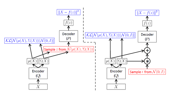
In practice, to ensure that gradients flow properly through the network, we use something called the reparametrization trick; rather than sampling directly from the distribution produced by Q, we instead randomly sample from N(0, 1), and scale the sample with μ(x) and Σ(x). This ensures two things: first, that sampling from the distribution N(z; μ(x), Σ(x)) in fact drives the reconstruction of X, ensuring that we are truly learning a distribution as a representation; second, that gradients can flow unimpeded by a stochastic layer.
Thus, by formulating the problem in this way, variational autoencoders turn the variational inference problem into one that can be solved by gradient descent. More importantly, note that the decoder network P also serves as a generative model — it can generate new samples given an input from N(0, 1).
Introduction (II): Representation Learning
A representation, intuitively speaking, is a low-dimensional analogue of something high-dimensional that captures the “essential” components of the initial object. Representation learning is therefore analogous to feature learning, where the goal is to learn the most “representative” features directly from the data. The key fact about a representation is that it can reduce the dimensionality of what you are studying while preserving key relationships between points or groups of points that exist in the original dataset.
One question worth asking is why we care about learning good representations of data — wouldn’t it better if we just used the real data? This can fall short for two main reasons — either due to the initial measurement space being noisy, or prohibitively high dimensional.
A quick example would be that of images — consider a simple computer vision application where the input images are of size 400 x 400. Naively, if we were to flatten the image into a vector, this would give us a 160,000-dimensional representation of this particular image. This is an extremely high dimensional object, and the computational costs associated with training a model with such a large input size are not trivial — matrix multiplication alone scales as O(n³).
If we could condense this to, say, a 100 dimensions, that would remarkably speed up training and inference time. Learning good representations also lets us fully understand the nature of the data we are working with as well as its generative process — and as we have seen, variational autoencoders actually allow us to sample from the space of representations, generating new examples that we have not yet seen.
On that note, it would be great if our representations were in some sense disentangled. Concretely, assume we have some input X with dimensionality D and its representation Z with dimensional d such that D>> d. We would like it if we changed precisely one element of Z, then that would change precisely one “characteristic” of X. For example, if X constituted a set of images of human faces, then we would like it if Z represented the “essential” components of a human face, and that changing the value of one component of Z would be akin to, say, toggling a hairstyle on a given face.
Learning Disentangled Representations
Let us now take a look at how we can formalize disentanglement as a concept, and how we can go about learning disentangled representations. In the paper Isolating sources of Disentanglement in VAEs, Chen et al describe an approach that centers around a decomposition of the Evidence Lower Bound mentioned earlier, reproduced below:
This paper decomposes the right most term into the following 3 terms:
Where q(z|n) = q(z|xₙ) and q(z, n) = q(z|xₙ)p(xₙ).
The term of interest here is the second term, denoted the Total Correlation — it is intuitively easy to see why this term gets its name. If the components of z, denoted zᵢ were in fact independent, then we know from undergraduate probability that the joint distribution across all z should be equal to the product of the individual distributions of zᵢ, implying that the right hand side and the left hand side of component II would be the same. By the properties of the KL divergence, this term would then shrink to 0.
Inversely, the higher the correlation between the zᵢ, the more the true distribution over the Z would diverge from the factored space denoted by q(zᵢ), and the higher the KL-Divergence between the two terms. The authors claim therefore that penalizing this term results in learning disentangled representations.
The authors then substantiate this claim by pitting their model against a common variant of the VAE, the β-VAE. The β-VAE has exactly the same objective as a regular VAE, with an additional weighting of magnitude β on the rightmost term in the ELBO — the very same term that the Chen et al. paper decomposed. The Chen et al. variant — dubbed the Total Correlation VAE, or TC-VAE for short — placed the same penalty of magnitude β just on the TC term rather than on the entire expression.
Both the autoencoders were trained on a the CelebA dataset, and the results are below:
The figure displays traversals along specific attributes that were identified after-the-fact, with the bottom 5 rows corresponding to the Chen et. al variant (deemed the Total Correlation VAE, or TC-VAE for short), while the top 5 rows correspond to the beta-VAE. As can be seen just by visual inspection, the TC-VAE produces outputs that more faithfully adhere to the goal of changing single attributes when traversing a specific latent dimension. The disentanglement of the latent variables is clearly not perfect, but it is better than the beta-VAE, which frequently changes orientation and other visual features at larger scale than the TC-VAE. This seems to support the author’s claim that the Total-Correlation term does in fact influence the extent to which latent variables are correlated.
To summarize, the authors of this paper induced disentanglement in their learned representations by changing the functional form of the ELBO objective — quite interestingly, this method does not explicitly make demands of the geometry of the spaces the latent variables inhabit, but rather just forces the algorithm to learn representations that minimize a modified loss function. The next paper takes a slightly different approach by overtly demanding that each notion of similarity between training instances is geometrically disjoint from the others.
Learning disentangled subspaces with Triplet Information
As mentioned in the previous section, the TC-VAE paradigm imposes no constraints on the actual space occupied by the latent variables — that is to say, if we were to divide the latent space into subspaces and examine them individually, we would not a priori expect any meaningful structure to be encoded by these subspaces. A paper out of Cornell University’s Vision Lab entitled Bayesian Representation Learning with Oracle Constraints targets this issue, and makes these demands explicit..
The core idea of the paper is as follows — we can get some idea as to what the essential components (i.e. latent variables) of our data should be by assessing how similar or dissimilar two inputs are from each other. Formally, we can consider a triplet object (A, B, C) where A and B are similar and A and C are dissimilar. This seems like a reasonable approach. Consider the following contrived example: two bald men are certainly more similar to each other than a bald man and a woman with long hair, which would lead us to conclude that hairstyle is an essential component of human faces. This implies that if we had oracle information regarding the similarity or dissimilarity between input objects, we could very well begin to reason about their essential attributes.
There is one small catch, however — notions of similarity defined in this way might not be compatible with one another. Take another contrived example: consider a blue triangle, a red triangle, and a blue square. In terms of color the blue square and blue triangle are clearly similar, but in terms of shape the red triangle and blue triangle are more similar. These two definitions of similarity are therefore incompatible with each other, but they both clearly elucidate ‘essential components’ of the input objects, namely, their color and their shape.
The solution presented by the paper is as follows. Let X refer to the initial, D-dimensional data, and let Z refer to the d dimensional representation of X such that D >> d. Each notion of similarity — or query — implicitly defines a set of viable triplets (A, B, C) such that (A,B) are more similar than (A, C); denote this set TQ. The likelihood of a random triplet tᵏ belonging to TQ is then modeled as a Bernoulli distribution over the states True and False parametrized by the softmax function, as described below:
JS refers to the Jensen-Shannon divergence, which is akin to a symmetrized version of the KL divergence. In terms of probabilities, the full model for triplets is given by
The zᵢ in this case are the latent variables that give rise to the xᵢ, xⱼ, xₖ that actually constitute the triplet being monitored. Given this formulation, the paper then modifies the original generative model that VAEs attempt to approximate through variational methods as follows:
In doing so, the paper replaces the original generative model over x with a combined generative model over data points x and triplets t. The modified lower bound that is derived to reflect this change also displays this clearly:
Note again that this is the exact same evidence lower bound as in the case of VAEs, but with the addition of the rightmost term, which maximizes the log-probability of obtaining the triplet tₖ given the k-th draw of latent variables zᵢ, zⱼ, zₗ. Intuitively speaking, our coordinate ascent will now maximize the probability of X given latent variables Z, while also maximizing the probability of the triplets generated from the latent variables being legitimate triplets. In doing so, this formulation effectively forces the learning of latent representations that generate data points that constitute valid triplets, and so the triplet information is encoded into the latent representation itself.
Having discussed how triplets are utilized to generate latent representations, it remains to be seen how conflicting definitions of similarity are encoded. To do so, the paper introduces masks. Masks are effectively defined as query-specific on-off switches that determine which coordinates within the latent representations zᵢ are actually utilized when performing any kind of similarity computation. This allows different combinations of coordinates within the latent space to represent different notions of similarity — formally speaking, each notion of similarity is projected onto its own subspace parametrized by the coordinate directions left on by the masking operation. As such, the triplet divergence term featuring a mask m pertaining to a query Q therefore has the following form:
where mₕ is the h-th component of m.
To summarize: this paper utilizes triplet information in conjunction with the query-specific masking operator to give each notion of similarity its own subspace — by modifying the ELBO to take into account the triplet information, it allows every notion of similarity to be encoded in its own subspace. The procedure for maximizing the ELBO can be done analogously to how it is done with variational autoencoders, i.e. by parameterizing q(z|x) and p(x) with neural networks and performing coordinate ascent. In doing so, this paper effectively leverages triplet information from possibly inconsistent sources to learn good representations that can then be traversed subspace by subspace.
This algorithm was run on the Yale Faces dataset — this dataset was constructed by taking individuals, setting them under a lighting rig, and taking pictures of their faces from multiple angles under multiple lighting configurations. Broadly speaking there are three defining factors to an image — the identity of the person, the azimuth (i.e. the lateral position) of the camera, and the elevation (i.e. the vertical position) of the camera. These three defining factors were also used to define a notion of similarity, and so construct triplets. Each notion of similarity was encoded into its own subspace and projected into 2d via t-Stochastic Neighborhood Embedding. As shown below, the results obtained by running this algorithm on this dataset are striking:
As we can see, the algorithm managed to effectively recover different notions of similarity with some geometric intuition. Identities and degree of elevation were well clustered, while the azimuth — being a smoothly varying quantity — was appropriately represented as a smooth, contiguous surface. In the paper, the authors even provide examples of image arithmetic, where aspects of one image were fused with another to create an image with aspects of both in a representative fashion (i.e. shadows from image A plus identity from image B resulted in an image with the identity of image B but the shadows of image A). Clearly, this approach has led to a well-disentangled representation that is semantically meaningful.
One clear drawback of this approach, however, is that the queries themselves need to be decided a-priori so that they can be then used to generate the triplets. In some sense this model only disentangles the latent space to the extent that the user specifies what components exactly should be disentangled.
Conclusion
In this blog, we’ve taken a look at variational autoencoders, and how they use neural networks to effectively bridge the gap between representation learning and variational inference by reducing the variational problem to an optimization problem that can be well-approximated through gradient descent. We’ve also taken a look at how the learnt representations can be disentangled through two very different approaches, each with their own pros and cons.
One key question that remains to be answered is this: why do we bother with the variational setting at all, rather than utilizing a simple deterministic autoencoder? Utilizing a variational autoencoder with a Gaussian prior in some sense enforces a prior on the structure of the latent space, ensuring that we transition smoothly between different pockets of the latent space. This structure is absent in conventional autoencoders. Additionally, variational autoencoders are generative models and so allow us to sample new examples, while allowing us to encode multiple notions of similarity quite well.
Directions for future research
VAEs are an open area of research, with many questions left to be answered. These include:
- Imposing different non-Gaussian priors on the latent space.
- Replacing the KL divergence with different f-Divergences, such as the JS-Divergence.
- Improving the “fuzziness” of VAE reconstructions, in contrast to GANs.
- Imposing metric losses directly on the latent variables to meaningfully cluster the latent space.
- Stochastic Dimensionality: there has been some work on using stick-breaking priors in conjunction with VAEs to let the data “determine” the number of latent dimensions required.
References
- Tutorial on Variational Autoencoders: Carl Doersch
- Isolating Sources of Disentanglement in Variational Autoencoders: Chen. et al
- Bayesian Representation Learning with Oracle Constraints: Karaletsos et. al

